The total home-game attendance for major-league baseball is the sum of all attendees for all stadiums during the entire season.The home attendance (in millions)for a number of years is shown in the table below. $$\begin{array}{cc}\text{ Year }& \text{ Home Attendance (millions) }\\ 1978& 40.6\\ 1979& 43.5\\ 1980& 43.0\\ 1981& 26.6\\ 1982& 44.6\\ 1983& 46.3\\ 1984& 48.7\\ 1985& 49.0\\ 1986& 50.5\\ 1987& 51.8\\ 1988& 53.2\end{array}$$ a)Make a scatterplot showing the trend in home attendance.Describe what you see. b)Determine the correlation,and comment on its significance.
c)Find the equation of the line of regression.Interpret the slope of the equation.
d)Use your model to predict the home attendance for 1998.How much confidence do you have in this prediction? Explain.
e)Use the internet or other resource to find reasons for any outliers you observe in the scatterplot.

a) 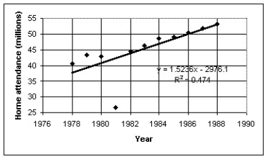The data show a strong association with the exception of a conspicuous outlier at year 1981. b)R2 = 0.474.The correlation coefficient is not very large even though the trend looks strong.The conspicuous outlier at year 1981 is exerting leverage on the model. c)y = 1.5236x - 2976.1.The home attendance is increasing by about 1.5 million per year. d)y(1998)= 1.5236 ∙ 1998 - 2976.1 = 68.1 million.There are good reasons to have only weak confidence in the prediction.First,the outlier at year 1981 demonstrates that the actual data is subject to some unusual disturbance.Second,this outlier is exerting a large influence on the slope of the model,drawing the model toward it.Third,1998 is fairly distant from the most recent year in the data,1988,which means that the model is forecasting fairly far into the future.This always leads to weaker confidence in the prediction. e)The 1981 season was shortened due to a players' strike.